Conversion
How a raw ADC code becomes a temperature, with integers only: the pipeline, the divider, the three ways to describe a part, how accurate each is, and how to make a table from any description or from a vendor list.
Datasheet sections this page relies on
From Public references n/a n/a:
- Beta equation and the B25/85 pair: Beta model, 1/T = 1/T0 + ln(R/R0) / B, p. 1
- Steinhart-Hart and the table tool: Steinhart-Hart, 1/T = a + b ln R + c ln(R)^3, p. 1
- Voltage divider and the series resistor: Divider, V = V_s R_n / (R_s + R_n), p. 1
All of them, with the driver API for each: Datasheet map.
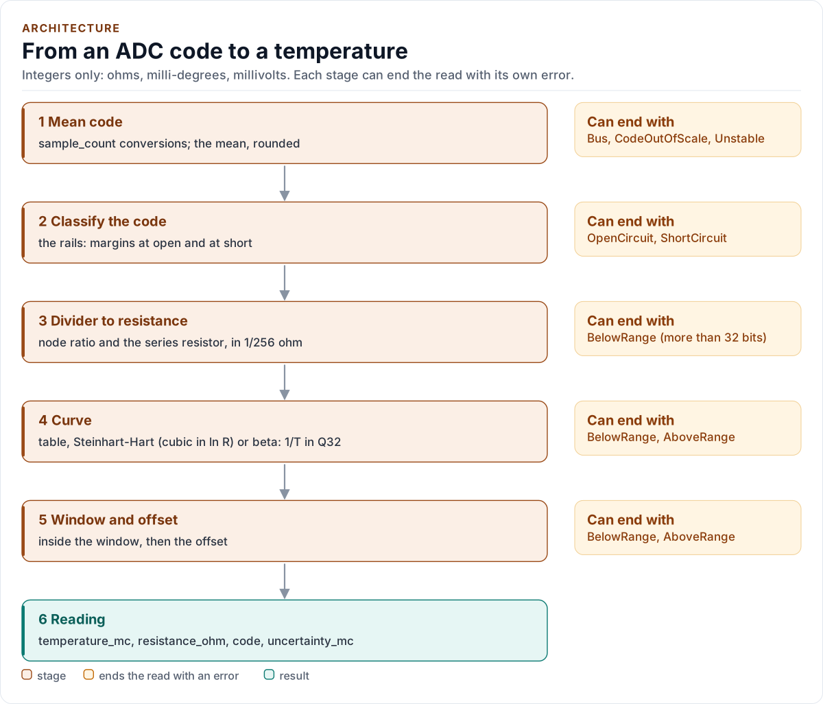
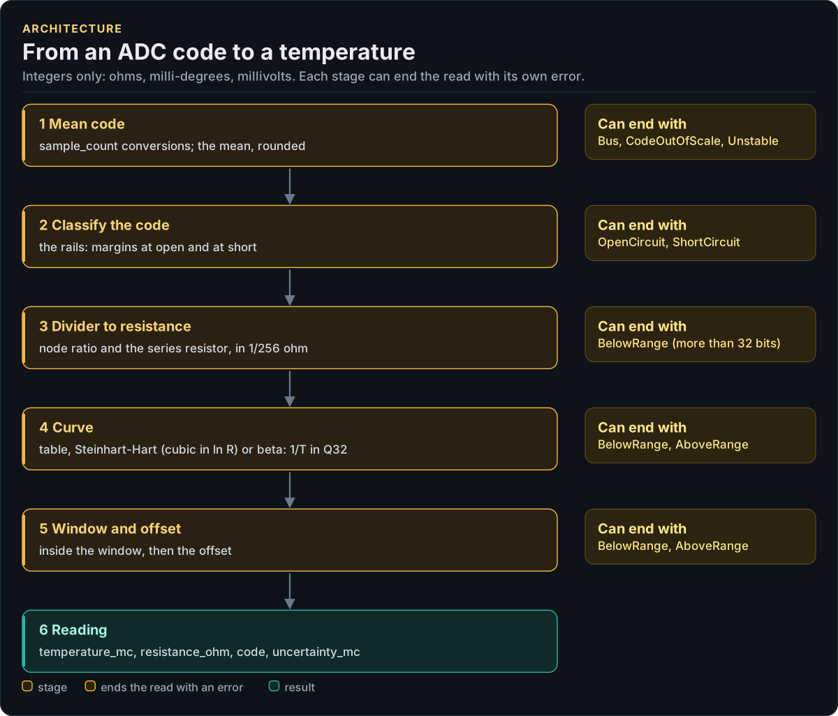
Figure description and sources
Top to bottom, each arrow hands one number to the next stage. Read() takes sample_count codes and their mean (the spread check can stop it as Unstable). The mean code is classified: at or above 2^bits is CodeOutOfScale, a code in the margin at the open rail is OpenCircuit, one in the margin at the short rail is ShortCircuit; which rail is which depends on the divider side. The node ratio gives the thermistor's resistance from the series resistor, in 1/256 ohm. The resistance goes through the curve: a table (a bounded binary search, then linear interpolation in ln R) or Steinhart-Hart (a cubic in ln R) or the beta equation (1/T in Q32), any of them with no floating point and no library. The temperature must lie inside the window; the offset is added last. The uncertainty bound is computed from the same code. The stages are the functions of inc/ntc_thermistor_conversion.hpp.
Drawn from: inc/ntc_thermistor_conversion.hpp ConvertCode(); inc/ntc_thermistor_conversion.hpp FineOfCode(); inc/ntc_thermistor_conversion.hpp CurveTemperature(); figure module docs/diagrams/figures/conversion-pipeline.py.
All quantities are integers: resistance in ohms, temperature in milli-degrees Celsius, voltage in millivolts,
tolerance in parts per million. There is no floating point and no library call (libm is not linked); the
logarithm is an integer function, Ln16(), accurate to within one unit of 2^-16 neper over 1 to 2^64 - 1 (measured
0.77 unit), with its own test.
1. The code
Read() takes sample_count conversions, each checked: a code at or above 2^adc_bits is CodeOutOfScale. The mean
is (sum + count / 2) / count. If max_spread_codes is set and the largest sample minus the smallest is more, the
reading is Unstable. The code is a number of ADC steps; the driver treats a node ratio as code / 2^bits (one step
different from code / (2^bits - 1), which is inside the quantisation; pinned by a test, not verified on hardware).
2. Classifying the code
Before any arithmetic the driver rules out the codes that cannot be a thermistor:
| Code | Low-side divider | High-side divider |
|---|---|---|
Within open_margin_codes of full scale |
OpenCircuit |
ShortCircuit |
Within short_margin_codes of zero |
ShortCircuit |
OpenCircuit |
The margins belong to the fault, not to the rail: they swap with the topology. When the reference is above the divider
supply the node cannot read above 2^bits * supply / reference: the margin at the open (or short) rail is counted
from that code, not from the converter's top code. With 12 bits, a 3300 mV reference and a 3000 mV supply the node
tops out at code 3723, so with the default margin of 2 the codes from 3720 up are the fault. The margins are in codes,
so on a 20-bit or wider converter two codes are noise: choose them from the noise of the node (see
Reference and supplies).
3. From the node to a resistance
With r = code / 2^bits (or code / 2^bits * vref / supply when the reference and the supply differ):
The driver carries the resistance in 1/256 ohm ("fine ohms") rounded to nearest. Whole ohms would cost as much as
an ADC step at the hot end of a low-resistance part. A resistance that does not fit 32 bits is BelowRange; zero is
AboveRange.
4. From a resistance to a temperature
A curve is exactly one of a table, Steinhart-Hart coefficients, or R25 and B. All are data: a non-empty table
selects table mode, otherwise a non-zero sh_b_e15 selects Steinhart-Hart mode, otherwise it is beta mode.
Table mode
2 to 256 rows, any spacing, resistance strictly falling as temperature strictly rises. The driver finds the segment by a binary search of at most 8 steps, then interpolates linearly in ln R, which follows the real curve far better than linear in R:
Above the first row's resistance is BelowRange (colder than the table), below the last row's is AboveRange. There
is no extrapolation. A row is exact: a resistance equal to a row's returns that row's temperature. An end of the table
is a hard edge: a node a fraction of an ADC step beyond the first or last row is a range error, not the end
temperature. Extend the table (the generator takes --from and --to) so that the part's rated range lies inside it.
The step rule. The interpolation error grows with the square of the row spacing. For tables built from a beta
curve the worst error over a segment was measured at 0.105 K for 10 degree rows, 0.027 K for 5 degree rows and
0.007 K for 2.5 degree rows, so it is bounded by 0.0013 * step^2 + 0.003 kelvin, step in degrees (the model pins
this in tests/test_model.cpp). A table with rows every 5 degrees or less is within about one ADC step of the curve on
a 12-bit ADC; rows every 10 degrees or more make the table the dominant error.
Steinhart-Hart mode
The coefficients are Curve::sh_a_e15, sh_b_e15 and sh_c_e15, integers in units of 1e-15 per kelvin: a vendor's A =
0.8767633e-3 is 876'763'300'000, B = 2.527899e-4 is 252'789'900'000, C = 1.906681e-7 is 190'668'100. A non-zero
sh_b_e15 selects the mode; r0_ohm, b_kelvin and b_tol_ppm must then be 0 (one description only). Validate()
requires bounded coefficients, 1/T rising with ln R over the whole resistance range (B > 0, and B + 3 C ln(R)^2 > 0 at
the largest ln R), and a window, as for beta mode: the polynomial extrapolates. The maths is Q16 arithmetic on Ln16():
the cube is formed in two Q16 products and the temperature is 10^18 / (1/T in 1e-15) in milli-kelvin, so it is
measured within 5 mK of the equation over -40 to 150 degrees Celsius (10 mK in a randomised check of other coefficient
sets up to 300 degrees Celsius, against an independent Python evaluation). An inverse that is not positive is
AboveRange. The coefficients carry no tolerance: put the fit's error into curve_error_mc. This is the
three-coefficient form with R in ohms. A vendor that publishes a four-term polynomial, ln R of R in kilo-ohms or
another R0 normalisation needs its coefficients converted, or a table: tools/ntc_table.py list makes one from the
vendor's own resistance and temperature list, with no model at all.
Beta mode
R0 is r0_ohm at ref_temperature_mc (25 degrees Celsius for nearly every part) and B is b_kelvin; the sum is
computed in Q32 fixed point. Beta mode requires a window, min_temperature_mc and max_temperature_mc: the
equation is a two-point fit and extrapolates without complaint, so the driver will not guess the range for you. A
temperature outside the window is BelowRange or AboveRange. b_t2_mc records the second temperature of the B pair
you took B from (85 degrees Celsius for B25/85); it is validated but does not enter the arithmetic.
Beta fits a real part exactly at the two temperatures of its pair and drifts away from them. Use it when the part's datasheet gives only R25 and B, over a range near the pair; use a table when it gives a table.
5. Window, offset, bound
The temperature must lie in [min_temperature_mc, max_temperature_mc]; then offset_mc is added (saturating).
Reading::uncertainty_mc is a worst-case linear sum, at least 1 and saturating, of:
- the tolerance of R (
r_tol_ppm): the temperature atR * (1 + tol)andR * (1 - tol), rounded outward; - the same for the series resistor (
series_tol_ppm); - the tolerance of B (
b_tol_ppm), in beta mode and in table mode:T^2 * |1/T - 1/T0| * tol, which isT^2 * |ln(R / R0)| / B * tolfor a beta curve and uses the table's own implied B at this point for a table (T0isref_temperature_mc); it is zero at the reference temperature and about 1.3 K at 125 degrees Celsius for 1 %; - the error of the curve itself (
curve_error_mc): the fit error of Steinhart-Hart coefficients, or the interpolation error of a table (the generator prints it); - one ADC step, from the neighbouring codes.
A tolerance of 0 means "not declared" and adds nothing; with nothing declared the bound is one converter code. It is a bound on the declared tolerances, not a guarantee about the part: the tolerance of R is applied as the same ratio at every temperature, whereas a vendor's tolerance grows away from 25 degrees Celsius (declare the largest). It does not include self-heating, the ADC's own gain and offset errors, or a filter that has not settled.
Beta against a table, the same part
The case for tables, on the worked example (the rows of the example preset, unverified, against a beta curve with B25/85 = 3435 K, R25 = 10 kOhm; error = beta minus table):
| Temperature (degC) | Table (degC) | Beta (degC) | Beta error (K) |
|---|---|---|---|
| -35 | -35.03 | -31.12 | +3.88 |
| -20 | -20.02 | -17.50 | +2.50 |
| 0 | 0.01 | 1.12 | +1.12 |
| 25 | 25.00 | 25.00 | 0.00 |
| 50 | 50.00 | 49.58 | -0.42 |
| 85 | 85.00 | 85.01 | +0.01 |
| 100 | 99.99 | 100.48 | +0.48 |
| 125 | 124.92 | 126.60 | +1.60 |
| 145 | 144.99 | 147.95 | +2.95 |
Beta is right where its pair is and wrong by a few kelvin at the ends. The table follows the part. The same conclusion holds for any part whose real curve is not a single beta: see Worked example.
Making a table
A table is the form every part can take. tools/ntc_table.py makes one, checks it the way Validate() does, and prints
the interpolation error against the source curve:
# Steinhart-Hart coefficients (a datasheet's or a calibration's)
python3 tools/ntc_table.py sh 0.8767633e-3 2.527899e-4 1.906681e-7 --from -40 --to 150 --step 5 --name kMyPart
# R25 and B
python3 tools/ntc_table.py beta 10000 3950 --from -40 --to 125 --step 5
# A vendor's list: lines of "temperature_degC resistance_ohm"
python3 tools/ntc_table.py list vendor_table.txt --name kMyPart
It prints a constexpr array of TablePoint, then a comment with the row count, the range, and the measured
error at the middle of every segment. It exits non-zero when the table would be refused: fewer than 2 or more than 256
rows, a resistance that does not fall strictly after rounding to whole ohms, two rows whose logarithms agree to 2^-16,
a resistance that does not fit 1 to 2^32 - 1. --max-error K fails a table whose error is above K. Declare the
result as Curve{.table = kMyPart} (the rows must outlive the driver: a static constexpr array), and put the printed
error in curve_error_mc.
A worked check, for the part of the Worked example: the coefficients above, rows every 5 degrees
from -40 to 150, give 39 rows from 188 kOhm (-40) to 310 ohm (150) and a measured error of 0.040 K at the middle of a
segment (the step rule, measured on beta curves, says 0.036 K: a cubic fit is steeper at the hot end, so give the
printed figure to curve_error_mc rather than the rule). The CI test builds that table with the tool and checks that
Convert() on it follows the equation to 0.06 K (tests/generated/).
Those coefficients are a fit of a secondary listing of the table and deviate from its rows by up to 0.41 K (they reproduce the nominal 25 degree row to 0.01 K). Use the coefficients of your own datasheet. A parallel resistor across the thermistor (a common linearisation) is not a model of the driver: tabulate the network, that is, give the tool the parallel resistance for each temperature in a list.
Next: Presets.